Lab 3 -- Numerical Methods
This lab is about basic numerical methods for computation of solutions to first-order ODE's. You will again need to be familiar with dfield6.
Pre-lab: Do all this stuff for practice. I will not need it turned in.
Note: You'll be making functions (saved as M-files, e.g., "my_function.m") in this lab. If you would rather keep these files around so that you can adjust them later on and work in the same directory throughout the course, then make sure you save your M-files to your home drive. Then, to be able to use those files, load "File | Set path ..." and include that directory in your path. Then you can work with your saved files again.
Overview: Euler, Improved Euler, and Runge Kutta are all names of different
numerical methods used to approximate solutions to first-order ODE's. We will
take a look at how the Euler and Improved Euler methods work. (If you want to
see Runge Kutta, try CS 414.)
To start, here's how the Euler method works:
You begin with an initial point of data, (t, y), and you know that y' = f(t, y).
You'll also have a step size, h. You want to find a solution curve through (t,
y). You do this by computing (t_next, y_next).
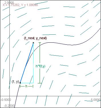
You compute t_next and y_next as follows:
t_next = t + h
y_next = y + h*f(t,y) [where f(t,y) = y'.]
Then you repeat the process, except now you use (t_next, y_next) as your new (t,
y). Connect the dots between the (t, y) points and you have the Euler
approximation of the solution curve.
Euler and Improved Euler methods are covered in your text on pp. 452-57.
Let's look at the exercises:
- As per directions, exit dfield, re-enter, plot y' = y + t, 0 <= t <= 3,
0<= y <= 8. Type 'hold on' in the command screen. Now enter the command for
graphing the simple Euler approximation. Remember that the syntax for the 'eul'
command is eul('function_name', [t_min, t_max], y_min,
step_size)." To set the results to a vector, you use "[t, y] = eul(...)"
Then plot(t,y).
Here's how you get from (t,y) to the next point, (t_next, y_next):
y' = f(t,y)
t_next = t + h
y_next = y + h*f(t,y)
I'll give the first couple steps to the arithmetic here:
Our initial point is (t,y) = (0,0). The slope of our line coming from that initial point is y'(initial point) = y'(0,0) = y+t | (y=0, t=0) = 0 + 0 = 0. This gives you the slope of the first line segment in the Euler approximation. Now find the point that this line connects to. You will simply follow a line from your starting point, (0,0), to a new point that increases by .5 in the t-direction and has slope = y'(0,0) = 0. I.e. it has no change in the y-direction.
Our initial point was (0,0). So the new point is (initial value of t + change in t, initial value of y + dy/dt|(initial point)*change in t). That is, our second point is (0,0)+(.5, 0*.5) = (.5,0).
Now our initial point is (.5,0). The slope of the line segment coming from that point is y'(.5,0) = .5 + 0 = .5. Our third point will then be (.5,0)+(.5, .5*.5) = (1,1/4). Find the slope of the segment coming out of this point and you will have all you need completed for this problem. Show these computations and try to show me that you understand what you're doing here. - This works roughly like the above problem, except now we're using the
Improved Euler method. This method is more accurate, and more complicated. The
MATLAB function you use here is 'rk2' instead of 'eul.' Improved Euler takes
us from one point (t,y) to (t_next, y_next) as follows::
Step size = h
y' = f(t,y)
m_1 = f(t,y)
m_2 = f(t+h, y + h*f(t,y))
t_next = t + h
y_next = y + (1/2)*h*(m_1 + m_2)
To do the Improved Euler's method, you will again start at your initial point, (0,0) in this case. Find the slope at this initial point, i.e., y'(0,0). Let m = y'(0,0). Then find out the point that this line would connect to, if you were to carry forward with the simple Euler method. Don't draw a line to that point. Instead, just evaluate y' at that point. Set y' at that point equal to n. Now the real slope that you use is the average of m and n, (m+n)/2. Follow a line of slope (m+n)/2 for a distance of .5 in the t-direction. Then you will have your new point. You will repeat the process from there.
Here's the first step:
y' = f(t, y) = y+t
h = 0.5
(t, y) = (0,0)
m_1 = f(t,y) = f(0,0) = 0 + 0 = 0
m_2 = f(t+h, y+h*f(t, y) )
= f(h, 0+h*(0)) = f(0.5, 0) = 0.5
t_next = t + h = 0 + h = 0.5
y_next = y + h/2*(m_1+m_2)
= 0 + (0.5)/2*(0 + 0.5)
= (.5)^2/2 = 1/8 = .125
So now (t_next, y_next) = ( 0.5, 0.125 ), and we repeat the process. The slope at this point is y' = f(0.5, 0.125) = 0.625. Now find the other slopes.
- Plot the solution in dfield. Then you find the error. You do this
by eyeballing your dfield6 plots: look at the Euler's method
approximation and the Improved Euler's method approximation, and see where
they are furthest away from the actual curve. The distance between the
approximations and the actual curve at a point of t is the
error of t. Find this for both Euler's and Improved Euler's methods.
- Make the M-file that they describe, with the text:
function yprime = zz(t,y)
yprime = (3-y)*(y+1)
Save this file. Whatever directory you save it into, make sure that it is in your MATLAB path. (You can adjust this by going to "File|Set Path ..." and then clicking "Add path"....)
Now plot the Euler approximation, with step size 0.5, and using 'zz' as your function, with initial values [0,0]. Plot this and explain the zig-zags in your graph. (The approximated solution crosses over the line y = 3, which is not possible for the real function. Perhaps the Euler line segment rode too far off on a tangent? Explain why this happens.) It asks what the significance of y = 3 is. It should be pretty clear by looking. Explain the difference in slopes above and below this line.
- Do the graphing listed by this problem. The problem with the Euler
approximation will be obvious. Explain this problem. Change the step size
until the problem gets better.
- Do the same for the Improved Euler method.
- Same again, but type 'rk4' in place of 'rk2.'
- Write your conclusions here. For (a), it should be fairly clear which
methods are best and which are worst. Give your thoughts for question
(b).
That's it for this lab.