Lab 11 -- The Pendulum
Lab 11 (click here for pdf) considers the following model of pendulum movement:
y'' = - (g / L) *sin(y).
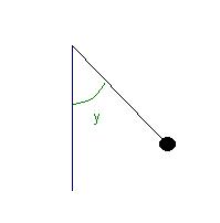
Here y is an angle, the angle that the pendulum makes with the vertical, and
not the vertical or horizontal position of the pendulum. For this lab we are
going that L = g / seed, and which simplifies the pendulum system to be
y'' = -(seed)*sin(y). (1)
On to the problems:
- Construct a first order system equivalent to y'' = -(seed)*sin(y), letting v = y'. Now find the equilibrium points (there are an infinite number of them) by solving for y' = v' = 0. Then use pplane to plot this system's phase portrait.
- Look at your pplane portrait to answer the first question. [That is, is (0,0) a saddle, sink, source, center?] Prove your answer using eigenvalues of the Jacobian matrix at (0, 0). Plot the linearized solution in pplane and notice the similarity of the linearized and actual systems around the equilibrium point.
- Note that (pi, 0) seems to be a different kind of equilibrium point. What
kind is it? Now use the Jacobian matrix evaluated at another equilibrium
point, (pi, 0), and use its eigenvalues to prove that the equilibrium point
actually is the kind of eq. point you said it was.
- Enter into pplane the system such that X' = AX, where A is the Jacobian matrix evaluated at (pi, 0) and compare the behavior of this system around (0, 0) to the behavior of the original system around (pi, 0).
- After entering this system, you'll then do the second part, involving "Plot stable and unstable orbits." Remember, when answering this question, that the straight line solutions are of the form x(t) = ci*e^(lambda_i*t)*vi. Also, the real component of lambda_i tell you something about whether or not that solution converges or diverges from the equilibrium point. - Now reenter the system for equation (1) into pplane and follow the
instructions for "plot stable and unstable orbits."
- You can then draw the tangent lines to these stable and unstable orbits at (pi, 0) on your printout. (You may simply sketch these by hand.)
- Then find the slope of these tangent lines. (Just pick out a couple points along each line and use the old algebra formula for getting the slope from two points.)
- Now look at the straight line solutions from #3. (Note that you can find two points for each straight line solution by simply substituting two values of t into x(t) = ci*e^(lambda_i*t)*vi. You can use these two points, and the old algebra slope formula, to get the slope.) Show your computations. Are the slopes the same? - Follow the instructions for plotting solutions inside and outside the
separatrices with different initial conditions.
- Plot y vs. t for several of these orbits. Describe the motion of the pendulum for the different types of initial conditions. (When describing the motion of the pendulum over time, remember what y models in this system. y is the angle between the pendulum and the vertical axis, not the horizontal or vertical position of the pendulum (see above picture). What does this have to do with the periodicity of the position of the pendulum?) - When answering this question, assume that the child is initially sitting
sitting on the swing at an angle of zero with the vertical (i.e., the kid is
sitting straight under the swing set). At what angle does the child have
to get pushed over top the swing?
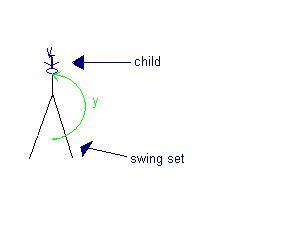
That is to say, what is y in the above picture? In any orbit on which the kid goes over the swing, y must go past the value for the picture above. Now look at your phase plane portrait. Look at the orbits where y = 0. What is the smallest value of v along y = 0 that falls on an orbit where y reaches the angle you see in the above picture? - Use the hint and remember that v' = y'' = -seed*sin(y). Remember also that
dy/dt = y' = v.
- Plug the values of y and v you're given into equation (3) on the lab handout to find C. Use fplot to plot the right hand side of equation (3). Remember that fplot plots functions, so you will need to plot both the positive and negative half of the left hand side, using fplot twice.
- In pplane, use the keyboard input option to plot the orbit corresponding to y(0) = 0 and v(0) = 1. - To find the formula, you will note that (pi, 0) is approached by the separatrices. Substitute (y, v) = (pi, 0) into equation (3) to find C. Then substitute the point (0, v0) into that equation to find v0. Explain why this is the exact same answer you got in #6.
- For small y, sin(y) ~= y. Thus the system can be approximated by y'' =
-seed*y. You'll here have to plot y'' = -seed*y in pplane.
- Find the general solution to this system. Find the period of this system.
- Get y vs. t graphs for different initial conditions, and compute the period of y on these graphs. Compare these periods with the predicted period. - In this problem, you will need to do the following to find the period of
the actual pendulum:
- Reenter the original system from equation (1) into pplane.
Then, for several values of v0,
- Use "keyboard input" to plot orbits through y(0) = 0, v(0) = v0.
- Get a plot of y vs. t for this orbit. Find the period, p.
After doing this for several values of v0, you will have a bunch of values of (v0, p). Use these and make a plot of period vs. v0. Does the period seem to depend on initial velocity? If not, at what value does the period seem to be significantly different from the value predicted by the linear approximation? - Just summarize according to the instructions.
That should be all for the labs.